Recipes for recording from a single analog source

The most basic use of picodaq

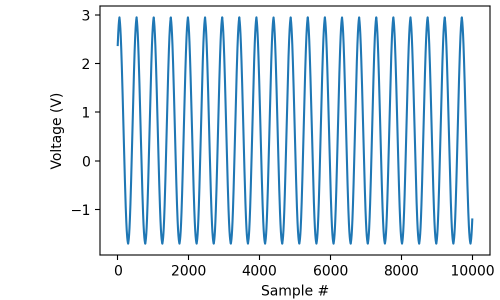
Read 200 milliseconds worth of data from channel “ai0” with a sampling frequency of 50 kilohertz and display the results using matplotlib:

from picodaq import *
import matplotlib.pyplot as plt

with AnalogIn(channel=0, rate=50*kHz) as ai:
    data = ai.read(200*ms)

plt.plot(data)
plt.xlabel('Sample #')
plt.ylabel('Voltage (V)')

In this case, I had an approximately 100-Hz sinusoidal signal connected to the input:

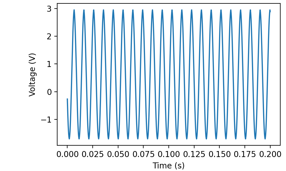
Retrieving timestamps

The read(...) function can also return timestamps along with your data:

with AnalogIn(channel=0, rate=50*kHz) as ai:
    data, times = ai.read(200*ms, times=True)

plt.plot(times, data)
plt.xlabel('Time (s)')
plt.ylabel('Voltage (V)')

Of course, you could have reconstructed the timestamps yourself using something like:

times = np.arange(len(data)) / 50000

but the earlier form generalizes a little better, as we will see below.

Reading more data

It is certainly possible to read a larger quantity of data with a single call to read(...), but you may want to do some online processing or show a progress bar.

import numpy as np

data = []
times = []
K = 25
with AnalogIn(channel=0, rate=50*kHz) as ai:
    for k in range(K):
        dat, tms = ai.read(20*ms, times=True)
        print(f"Progress {k+1}/{K}", end="\r")
        data.append(dat)
        times.append(tms)
print()
data = np.concatenate(data, 0)
times = np.concatenate(times, 0)

plt.plot(times, data)
plt.xlabel('Time (s)')
plt.ylabel('Voltage (V)')

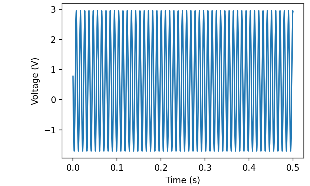
Notice that the timestamps are contiguous between read frames (as opposed to restarting from zero).

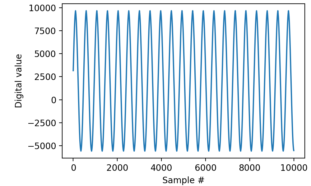
Retrieving raw binary data

On occasion, e.g. for debugging purposes, it may be useful to retrieve raw binary data.

with AnalogIn(channel=0, rate=50*kHz) as ai:
    data = ai.read(200*ms, raw=True)

plt.plot(data)
plt.xlabel('Sample #')
plt.ylabel('Digital value')