Recipes for using picoDAQ as a pulse generator
Outputting a sequence of pulses
To output a sequence of monophasic square pulses:
from picodaq import *
from picodaq.stimulus import Pulse, Train

pulse = Pulse(amplitude=1*V, duration=50*ms)
train = Train(pulse, pulseperiod=200*ms, pulsecount=10)
with AnalogOut(rate=50*kHz) as ao:
    ao[0].stimulus(train)
    ao.run()
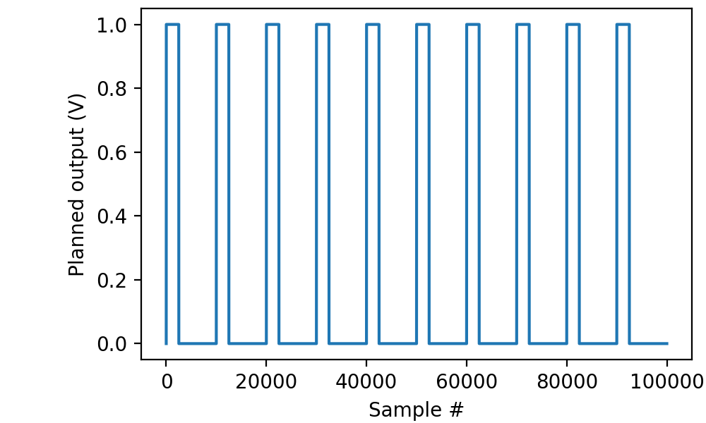
This outputs 10 pulses with amplitude 1 V and duration 50 ms to ao0, at a repetition rate of 5 Hz (programmed here as a period of 200 ms).
Note that it is not necessary to specify the output channel in the
AnalogOut constructor: the stimulus() call takes care of that.
Often it is desirable to visualize the programmed pulse train before actually sending it out:
import matplotlib.pyplot as plt
from picodaq.mockstim import mockstim

plandata = mockstim(train, rate=50*kHz)
plt.plot(plandata)
plt.xlabel('Sample #')
plt.ylabel('Planned output (V)')
Because PicoDAQ can simultaneously record and stimulate, we can readily verify that the output is indeed as advertised, by running the following code while a BNC cable connects ao0 to ai0:
with AnalogOut(rate=50*kHz) as ao:
    with AnalogIn(channel=0) as ai:
        ao[0].stimulus(train)
        data, times = ai.read(2*s, times=True)

plt.plot(times, data, '.-', markersize=1, linewidth=0.1)
plt.xlabel('Time (s)')
plt.ylabel('Voltage (V)')
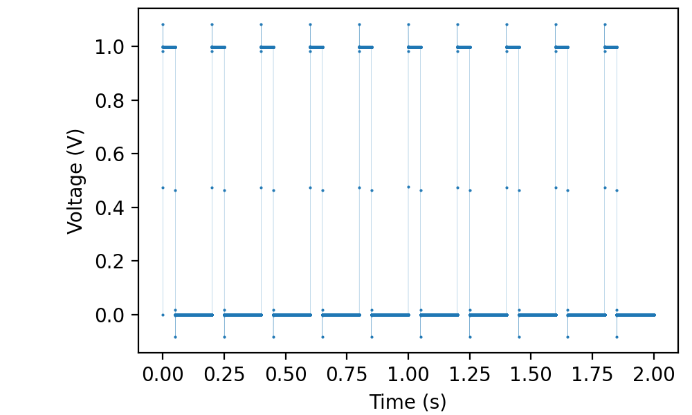
(Note the single-sample overshoots as the hardware attempts to make the sharpest possible square waves.)
The sampling rate is only set once on the first stream to be opened
(i.e., AnalogOut in the example above). Any secondary streams
automatically use the same sampling rate.
The act of reading from the input stream (ai.read(...))
automatically starts the output. Almost the same effect could be
obtained with
with AnalogOut(rate=50*kHz) as ao:
        with AnalogIn(channel=0) as ai:
            ao[0].stimulus(train)
            ao.run()
            data, times = ai.readall(times=True)
except that this causes the acquisition to end immediately after the end of the final pulse.
Outputting pulses of different shapes
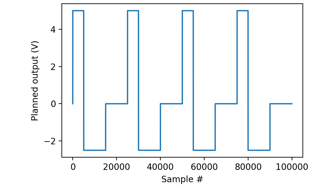
PicoDAQ can output pulses of a variety of shapes. For instance, here is how to generate asymmetric biphasic pulses:
from picodaq import *
from picodaq.stimulus import Square, Train

pulse = Square(amplitude=5*V, duration=100*ms,
               amplitude2=-2.5*V, duration2=200*ms)
train = Train(pulse, pulseperiod=500*ms, pulsecount=4)
with AnalogOut(rate=50*kHz) as ao:
    ao[0].stimulus(train)
    ao.run()
Again, we can visualize the pulses before actually generating output:
import matplotlib.pyplot as plt
from picodaq.mockstim import mockstim

plandata = mockstim(train, rate=50*kHz)
plt.plot(plandata)
plt.xlabel('Sample #')
plt.ylabel('Planned output (V)')
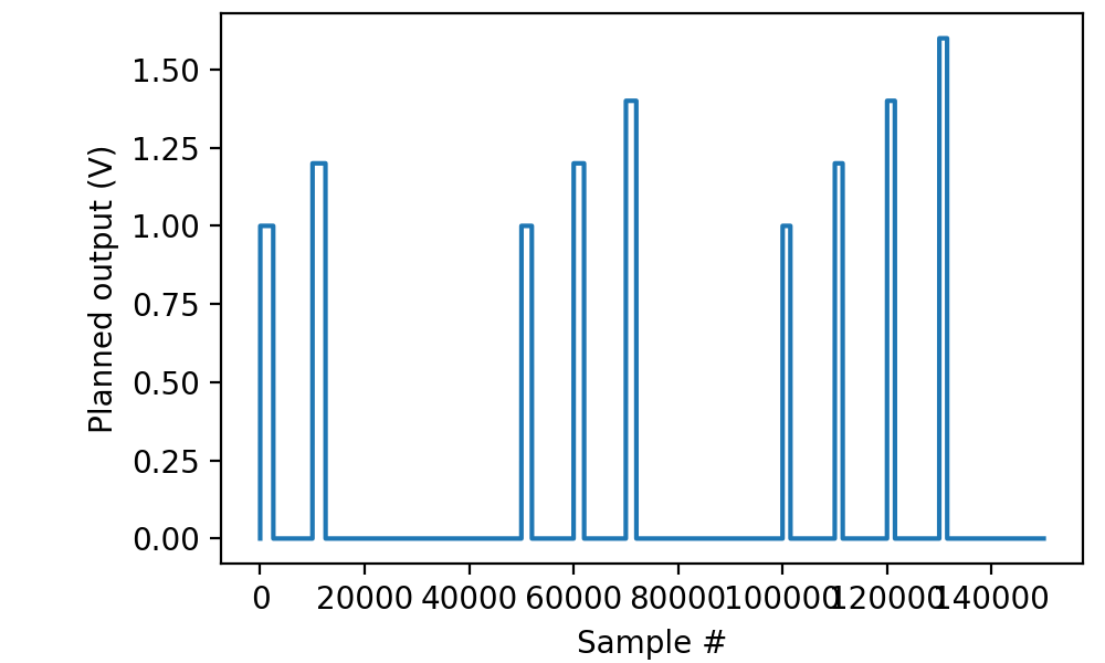
Outputting a sequence of pulses of increasing amplitude
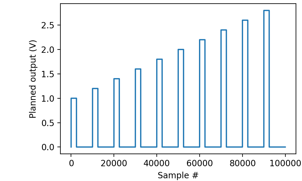
In the above examples, all of the pulse within a train were identical. PicoDAQ also allows us to vary them in a systematic fashion, for instance, increasing the amplitude by a constant amount for each subsequent pulse:
from picodaq import *
from picodaq.stimulus import Pulse, Train, Deltas

pulse = Pulse(amplitude=1*V, duration=50*ms)
delta = Deltas(amplitude=0.2*V)
train = Train(pulse, pulseperiod=200*ms, pulsecount=10,
              perpulse=delta)
with AnalogOut(rate=50*kHz) as ao:
    ao[0].stimulus(train)
    ao.run()
resulting in a stimulus sequence like this:
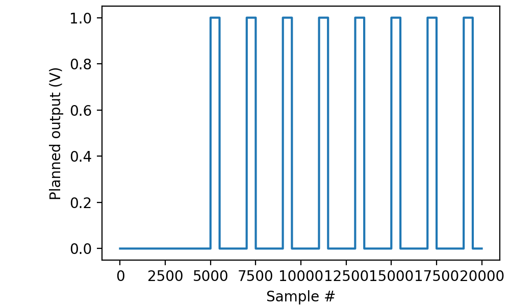
Outputting a sequence of trains with increasing pulse counts
Instead of a single train, PicoDAQ also allows us to define stimuli that comprise a series of trains, in which case it is possible to systematically vary parameters between trains:
from picodaq import *
from picodaq.stimulus import Pulse, Train, Series, Deltas

pulse = Pulse(amplitude=1*V, duration=50*ms)
pudelta = Deltas(amplitude=0.2*V)
trdelta = Deltas(pulsecount=1, duration=-10*ms)
train = Train(pulse, pulseperiod=200*ms, pulsecount=2,
              perpulse=pudelta)
series = Series(train, trainperiod=1*s, traincount=3,
                pertrain=trdelta)
with AnalogOut(rate=50*kHz) as ao:
    ao[0].stimulus(train)
    ao.run()
resulting in a stimulus sequence like this:
Note that both parameters pertaining to trains (e.g., the pulse count) and pertaining to the consituent pulses (e.g., the pulse duration) can be changed between trains. It is permissible to change a parameter both on a per-train and a per-pulse basis, in which case the changes are applied cumulatively.
Delaying the start of stimulation
Whether applying a single pulse, a train, or a series of trains, the
start of stimulation may be delayed relative to the start of the run
using the delay parameter to stimulus(...):
from picodaq import *
from picodaq.stimulus import Pulse, Train

pulse = Pulse(amplitude=1*V, duration=50*ms)
train = Train(pulse, pulseperiod=200*ms, pulsecount=10)
with AnalogOut(rate=10*kHz) as ao:
    ao[0].stimulus(train, delay=500*ms)
    ao.run()
The same delay parameter can also be passed to mockstim(...):
import matplotlib.pyplot as plt
from picodaq.mockstim import mockstim

plandata = mockstim(train, rate=10*kHz, delay=500*ms)
plt.plot(plandata)
plt.xlabel('Sample #')
plt.ylabel('Planned output (V)')
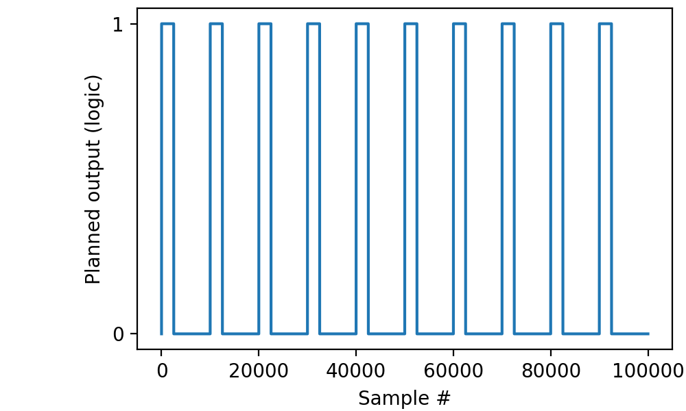
Outputting TTL pulses to a digital output
Unlike analog outputs, which admit a variety of pulse shapes, digital outputs only admit a single shape, TTL:
from picodaq import *
from picodaq.stimulus import TTL, Train

pulse = TTL(duration=50*ms)
train = Train(pulse, pulseperiod=200*ms, pulsecount=10)
with DigitalOut(rate=50*kHz) as do:
    do[0].stimulus(train)
    do.run()
Trains and series of trains can be constructed for digital outputs in
the exact same way as for analog outputs, except that there are fewer
pulse shape parameters that can be varied through Deltas.