Recipes for generating nonparametric (“sampled”) output
Although parametric output as considered in the previous two sections can be very convenient, not all cases are covered. For instance, picoDAQ’s pulse parametrization does not allow for sinusoidal frequency sweeps. For cases like that, and when the wave duration is too long to fit in the picoDAQ’s onboard memory, nonparametric, or continuously sampled, output offers a solution. You have two options: Either you precompute the entire waveform and offer it to picoDAQ in the form of a numpy array before starting the run, or you write a function that generates chunks of the waveform on the fly. We will show examples of both approaches.
Precomputed waveforms
The first step is to generate the waveform. For our example, we’ll
generate a frequency sweep using scipy’s sweep_poly function and inspect the result with matplotlib:
from picodaq import *
from scipy.signal import sweep_poly
import matplotlib.pyplot as plt
import numpy as np
f0 = 10 * Hz
f1 = 100 * Hz
dur = 1 * s
fs = 10 * kHz
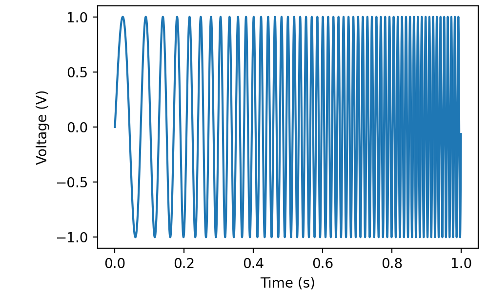
tt_s = np.arange(0, dur.as_('s'), (1/fs).as_('s'))
poly = [(f1-f0).as_('Hz') / dur.as_('s'), f0.as_('Hz')]
vv = sweep_poly(tt_s, poly, phi=-90)
plt.plot(tt_s, vv)
plt.xlabel('Time (s)')
plt.ylabel('Voltage (V)')
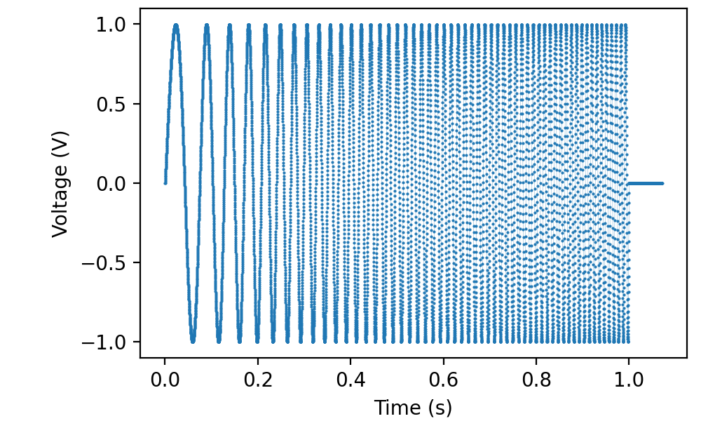
The result can be sent to analog output channel 0 using:
with AnalogOut(rate=fs) as ao:
    with AnalogIn(channel=0) as ai:
        ao[0].sampled(vv, scale=1*V)
        ao.run()
        data, times = ai.readall(times=True)

plt.plot(times, data, '.-', markersize=1, linewidth=0.1)
plt.xlabel('Time (s)')
plt.ylabel('Voltage (V)')
As per tradition, I connected ao0 to ai0, so we have a record of the produced waveform:
To be clear, the picoDAQ python library does not send the entire waveform to the device at the beginning of the run, but rather in small chunks during the run. As a consequence, the length of data that can be output in this fashion is only limited by the amount of memory in your computer.
Dynamic waveform generation
For exceedingly long waveforms, or in situations where the output has
to be adapted to external conditions, wave data can also be submitted
to picoDAQ on the fly. As a rather contrived example, the following
uses the real-time CPU frequency of your computer (as obtained by the
psutil module) to modulate a sine wave:
from picodaq import *
import psutil
import matplotlib.pyplot as plt
import numpy as np
f0 = 440 * Hz * 2**(-1 - 9/12) # C below middle C
fs = 48 * kHz
def getfreq():
fnow, fmin, fmax = psutil.cpu_freq()
return f0 * fnow / fmin
def produce():
ph = 0
t = 0*s
N = 256
while True:
f = getfreq()
dph = (2 * np.pi * f / fs).plain()
vv = np.sin(ph + dph*np.arange(N))
ph = (ph + dph*N) % (2*np.pi)
t += N/fs
yield vv
fff = []
ttt = []
t = 0
with AnalogOut(rate=fs) as ao:
with AnalogIn(channel=0) as ai:
ao[0].sampled(produce, scale=1*V)
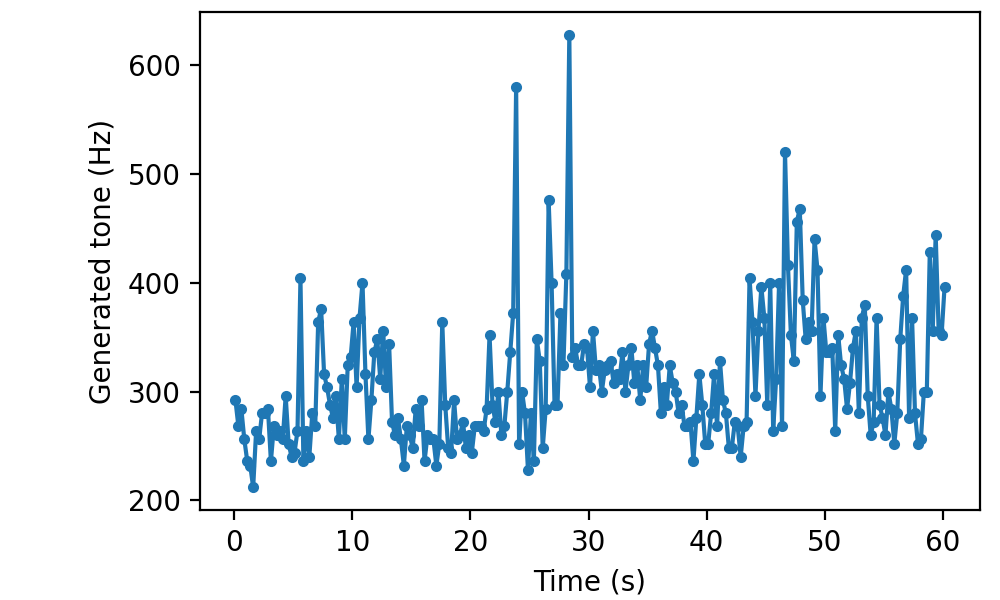
while t < 60:
vv, tt = ai.read(0.25*s, times=True)
pw = np.abs(np.fft.fft(vv))[:len(vv)//2]
fff.append(fs.as_('Hz')*np.argmax(pw)/len(vv))
t = np.mean(tt)
print(t)
ttt.append(t)
plt.plot(ttt, fff, '.-')
plt.xlabel('Time (s)')
plt.ylabel('Generated tone (Hz)')
Note that picoDAQ automatically refills the output buffer during
ai.read(...). If you don’t read, you will have to call
ao.poll() periodically to ensure the buffer stays filled.
The while t < 60 line in the example makes it stop after a minute,
but picoDAQ could go on all day if you let it. In particular, a simple:
with AnalogOut(rate=fs) as ao:
    ao[0].sampled(produce, scale=1*V)
    ao.run()
would run forever.
As always, it can be useful to visualize a segment of the generated data before sending it to the hardware:
from picodaq.mockstim import mocksampled

vvv = mocksampled(produce, scale=1*V, rate=fs, duration=10*s)
plt.plot(vvv)
plt.xlabel('Sample #')
plt.ylabel('Planned output (V)')
plt.xlim(50000, 60000)
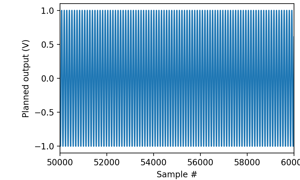
although in this particular case, the mockup is not entirely realistic, because it runs much faster and therefore does not capture a representative sample of cpu frequencies.