Recipes for recording from multiple analog sources

Reading a short segment from two channels

Read 200 ms worth of data from channels “ai0” and “ai1” with a sampling frequency of 50 kilohertz and display the results using matplotlib:

from picodaq import *
import matplotlib.pyplot as plt

with AnalogIn(channels=[0, 1], rate=50*kHz) as ai:
    data = ai.read(200*ms)

plt.plot(data)
plt.xlabel('Sample #')
plt.ylabel('Voltage (V)')

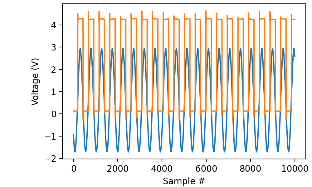
(The “TTL” output from my cheap function generator isn’t very clean.)

The resulting data is a T × C array where T is the sample count and C is the number of channels.

Retrieving time stamps

from picodaq import *
import matplotlib.pyplot as plt

with AnalogIn(channels=[0, 1], rate=50*kHz) as ai:
    data, times = ai.read(200*ms, times=True)

plt.plot(times, data)
plt.xlabel('Time (s)')
plt.ylabel('Voltage (V)')

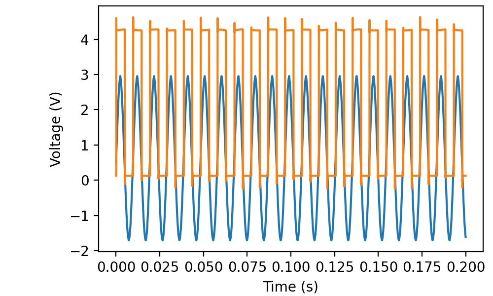
The times return value is still a simple T-vector.

Retrieving raw data

Retrieving raw data from multiple channels is equally straightforward:

with AnalogIn(channels=[0, 1], rate=50*kHz) as ai:
    data = ai.read(200*ms, raw=True)

The result is a T × C array of 16-bit integers.

Edge cases

It is perfectly legitimate to record a single channel in this way:

with AnalogIn(channels=[0], rate=50*kHz) as ai:
    data = ai.read(200*ms)

The result is a T × 1 array. In contrast, if you record a single channel with

with AnalogIn(channel=0, rate=50*kHz) as ai:
    data = ai.read(200*ms)

the result is a T-vector.

It is even OK to record from no channels at all:

with AnalogIn(channels=[], rate=50*kHz) as ai:
    data = ai.read(200*ms)

That takes 200 ms and results in a T × 0 array. This behavior is probably mostly useful if your use of AnalogIn is embedded in a function that receives its channels parameter from an external source.