Recipes for using triggers

Using triggers to start a recording

The trigger(...) method on AnalogIn and DigitalIn may be used to wait on a trigger condition before starting a recording:

from picodaq import *
import matplotlib.pyplot as plt

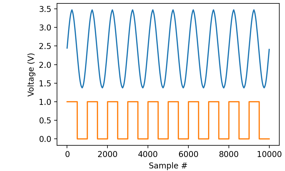
with AnalogIn(channel=0, rate=100*kHz) as ai:
    with DigitalIn(line=0) as di:
        ai.trigger(0, polarity=1)
        data = ai.read(100*ms)
        ddata = di.read(100*ms)
                    
plt.plot(data)
plt.plot(ddata)
plt.xlabel('Sample #')
plt.ylabel('Voltage (V)')

In this case, we wait until digital line “di0” goes high before recording 100 milliseconds from both “ai0” (connected to the main output of a function generator) and “di0” (connected to the TTL gate of the same function generator).

It is perfectly possible to trigger from a line that is not being recorded. For instance,

with AnalogIn(channel=0, rate=100*kHz) as ai:
     ai.trigger(0, polarity=1)
     data = ai.read(100*ms)

works just fine.

The trigger is edge-sensitive, not level-sensitive, meaning that it triggers on a low-to-high transition, not arbitrarily in the middle of a “high” stretch of the input.

It is equally possible to trigger on a high-to-low transition:

from picodaq import *
import matplotlib.pyplot as plt

with AnalogIn(channel=0, rate=100*kHz) as ai:
    ai.trigger(0, polarity=-1)
    data = ai.read(100*ms)
                    
plt.plot(data)
plt.xlabel('Sample #')
plt.ylabel('Voltage (V)')

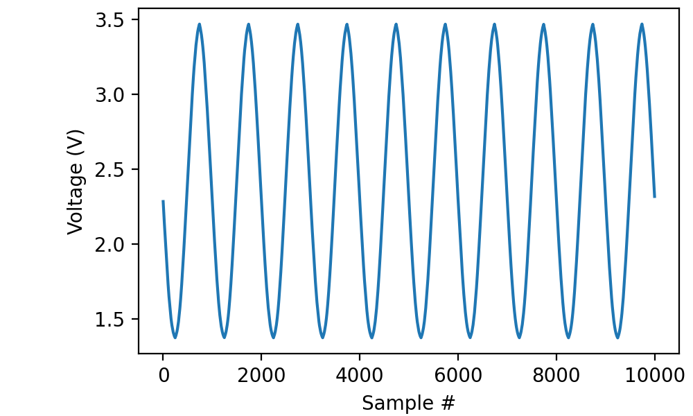
In this case I opted not to record the digital signal, but you can tell from the phase of the sine wave that we triggered on the falling slope of the digital signal.

Combining triggers with episodic recording

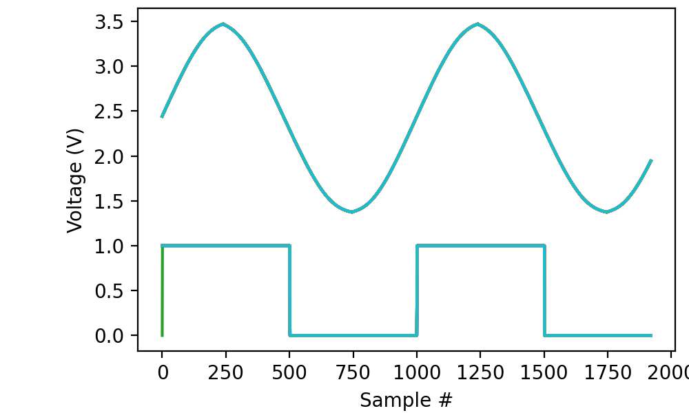
The combination of triggers and episodic recording is particularly powerful, as the start of each episode is delayed until the trigger condition is met.

import numpy as np

data = []
ddata = []
K = 20
with AnalogIn(channel=0, rate=100*kHz) as ai:
    with DigitalIn(line=0) as di:
        ai.episodic(duration=19*ms, period=0*ms)
        ai.trigger(0, polarity=1)
        for k in range(K):
            data.append(ai.read())
            ddata.append(di.read())
data = np.stack(data, 1)
ddata = np.stack(ddata, 1)
                    
plt.plot(data)
plt.plot(ddata)
plt.xlabel('Sample #')
plt.ylabel('Voltage (V)')

This captures 20 episodes of 19 milliseconds each. Each episode is triggered by the rising edge of the TTL signal from the function generator. As a consequence, all of the traces lie right on top of each other, neatly revealing that my old function generator produces ugly but consistent sine waves:

In the example above, I set period to zero, because I was happy to start the next episode on the first trigger after completing the previous episode. It is also allowed to set period to a larger value, to implement a “cooldown” period. E.g., period=1*s would ensure that the episodes are at least one second apart.