Recipes for using picoDAQ as a function generator
Outputting a sine wave
Like advanced traditional function generators, PicoDAQ can store arbitrary waveforms, and this is the most convenient way to produce sine wave output. The first step is to define the sine wave itself with a little numpy magic:
from picodaq import *
import numpy as np

f_out = 50*kHz
f_wave = 5*Hz
samples_per_period = int((f_out/f_wave).plain())

sinedata = np.sin(np.linspace(0, 2*np.pi, samples_per_period,
                              endpoint=False))
This defines a 5-Hz sine wave for use at 50-kHz sampling rate.
After that, we can visualize what the PicoDAQ intends to output:
import matplotlib.pyplot as plt
from picodaq.stimulus import Wave, Train
from picodaq.mockstim import mockstim

pulse = Wave(data=sinedata, scale=8*V)
train = Train(pulse, pulseperiod=1/f_wave, pulsecount=10)
plandata = mockstim(train, rate=50*kHz)
plt.plot(plandata)
plt.xlabel('Sample #')
plt.ylabel('Planned output (V)')
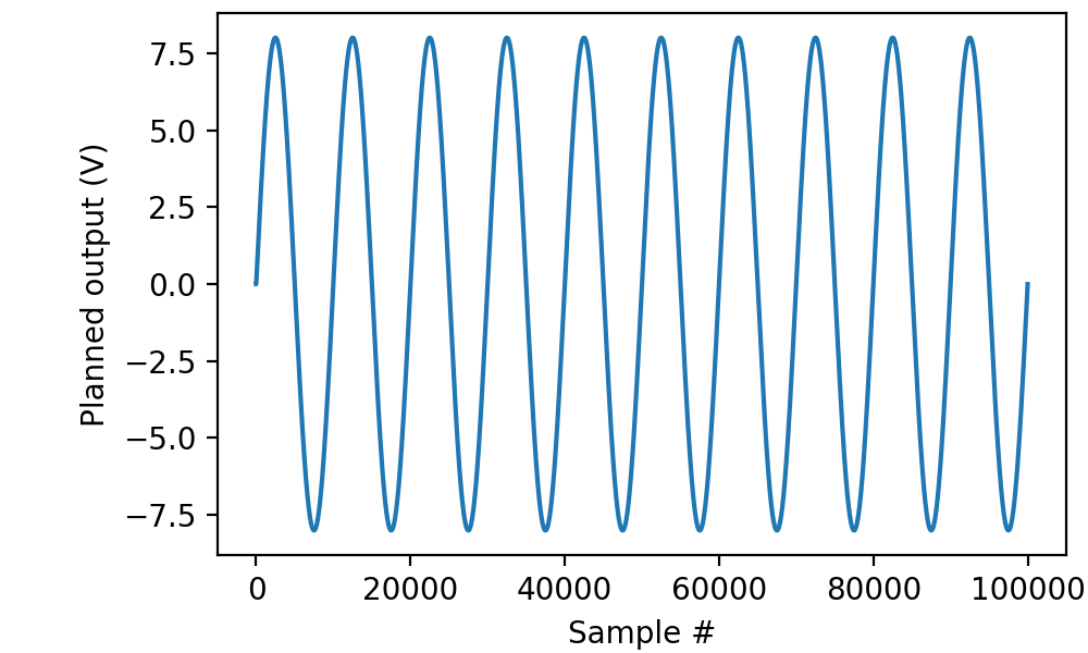
Note that the final amplitude of the sine wave is defined by the
scale parameter to Wave. As a useful convention, we defined the
core wave shape abstractly with amplitude 1. That way we can keep
track of physical units, despite the fact that numpy does not store
them in its vectors.
Actually sending this wave to the PicoDAQ uses the exact same code as for pulse output. In fact, from the perspective of PicoDAQ, function generator output is just pulse output with pulse period equal to pulse duration.
with AnalogOut(rate=50*kHz) as ao:
    with AnalogIn(channel=0) as ai:
        ao[0].stimulus(train)
        ao.run()
        data, times = ai.readall(times=True)

plt.plot(times, data, '.-', markersize=1, linewidth=0.1)
plt.xlabel('Time (s)')
plt.ylabel('Voltage (V)')
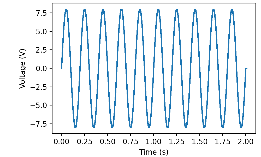
(As before, I connected a cable between ao0 and ai0 to record the signal.)
Naturally, wave shapes other than sines are equally possible. The only restriction is on the total number of samples in all waves simultaneously stored in the picoDAQ’s onboard memory. (If that restriction bites, consider using continuously sampled output.