Recipes for simultaneously generating multiple outputs
Simultaneously outputting two analog pulse sequences
Simultaneously generating output on two channels is done by assigning a stimulus to each of them:
from picodaq import *
from picodaq.stimulus import Square, Triangle, Train

pulse1 = Triangle(amplitude=0.7*V, duration=100*ms)
train1 = Train(pulse1, pulseperiod=200*ms, pulsecount=10)
pulse2 = Square(amplitude=1*V, duration=25*ms)
train2 = Train(pulse2, pulseperiod=100*ms, pulsecount=20)
with AnalogOut(rate=50*kHz) as ao:
    ao[0].stimulus(train1)
    ao[1].stimulus(train2)
    ao.run()
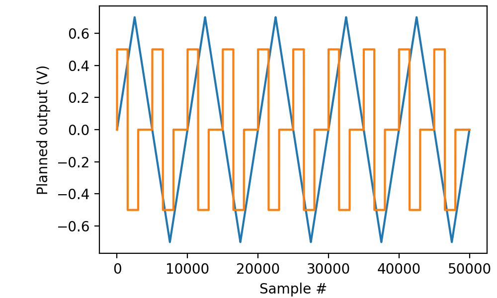
Visualizing these before sending them out is done separately:
import matplotlib.pyplot as plt
from picodaq.mockstim import mockstim

plandata1 = mockstim(train1, rate=50*kHz)
plandata2 = mockstim(train2, rate=50*kHz)
plt.plot(plandata1)
plt.plot(plandata2)
plt.xlabel('Sample #')
plt.ylabel('Planned output (V)')
As always, we can combine this with analog input to verify that the generated signals are as expected:
with AnalogOut(rate=50*kHz) as ao:
    with AnalogIn(channels=[0, 1]) as ai:
        ao[0].stimulus(train1)
        ao[1].stimulus(train2)
        ao.run()
        data, times = ai.readall(times=True)

plt.plot(times, data, '.-', markersize=1, linewidth=0.1)
plt.xlabel('Time (s)')
plt.ylabel('Voltage (V)')
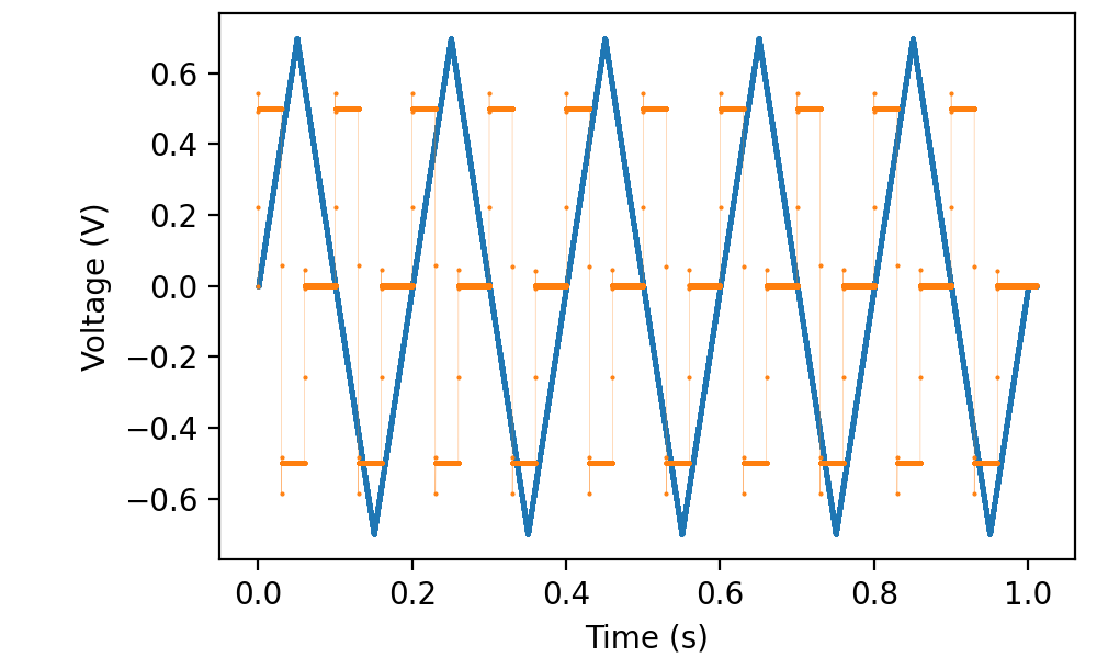
where I connected ao1 to ai1 in addition to connecting ao0 to ai0.
Simultaneously outputting two digital pulse sequences
In perfectly analogous way, we can send data to multiple digital outputs simultaneously:
from picodaq import *
from picodaq.stimulus import TTL, Train

pulse1 = TTL(duration=100*ms)
train1 = Train(pulse1, pulseperiod=200*ms, pulsecount=5)
pulse2 = TTL(duration=30*ms)
train2 = Train(pulse2, pulseperiod=100*ms, pulsecount=10)

with DigitalOut(rate=50*kHz) as do:
    do[0].stimulus(train1)
    do[1].stimulus(train2, delay=20*ms)
    do.run()
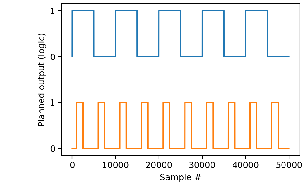
and visualize the stimulation plan before actually generating physical output:
import matplotlib.pyplot as plt
from picodaq.mockstim import mockstim

plandata1 = mockstim(train1, rate=50*kHz)
plandata2 = mockstim(train2, rate=50*kHz, delay=20*ms)
plt.plot(plandata1 + 2)
plt.plot(plandata2)
plt.xlabel('Sample #')
plt.ylabel('Planned output (logic)')
plt.yticks([0, 1, 2, 3], [0, 1, 0, 1])
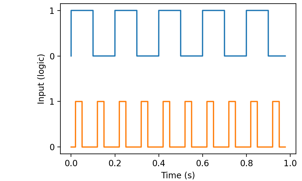
By connecting do0 to di0 and do1 to di1, we can verify that the output is as expected:
with DigitalOut(rate=50*kHz) as do:
    with DigitalIn(lines=[0, 1]) as di:
        do[0].stimulus(train1)
        do[1].stimulus(train2, delay=20*ms)
        do.run()
        data, times = di.readall(times=True)


plt.plot(times, data[:,0] + 2)
plt.plot(times, data[:,1])
plt.xlabel('Time (s)')
plt.ylabel('Input (logic)')
plt.yticks([0, 1, 2, 3], [0, 1, 0, 1])
Simultaneous analog and digital output
Mixing parametrized analog and digital outputs is done by creating
both AnalogOut and DigitalOut objects. As usual, we begin by
visualizing the planned pulse sequences:
from picodaq import *
from picodaq.stimulus import Triangle, TTL, Train
import matplotlib.pyplot as plt
import numpy as np

fs = 10 * kHz
apulse = Triangle(duration=50*ms, amplitude=1*V)
atrain = Train(apulse, pulseperiod=100*ms, pulsecount=9)
dpulse = TTL(duration=20*ms)
dtrain = Train(dpulse, pulseperiod=200*ms, pulsecount=5)

aplandata, att = mockstim(atrain, rate=fs, times=True)
dplandata, dtt = mockstim(dtrain, rate=fs, times=True)

plt.plot(att, aplandata)
plt.plot(dtt, -1.5 + .3*dplandata)
plt.xlabel('Time (s)')
plt.ylabel('Planned logic / voltage (V)')
plt.yticks([-1.5, -1.2, -1, 0, 1], ['Lo', 'Hi', -1, 0, 1])
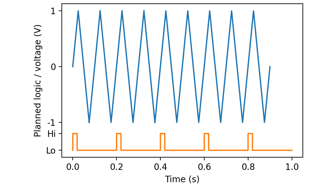
We ask for times to be returned from both mockstim calls,
because there is no assumption that the sequences are the same length.
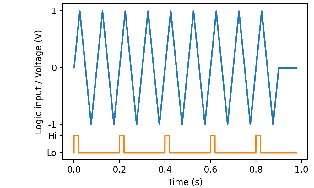
Then we connect do0 to di0 and ao0 to ai0 to verify that the output is as expected:
with AnalogOut(rate=fs) as ao:
    with DigitalOut() as do:
        with AnalogIn(channel=0) as ai:
            with DigitalIn(line=0) as di:
                ao[0].stimulus(atrain)
                do[0].stimulus(dtrain)
                ao.run()
                adata, times = ai.readall(times=True)
                ddata = di.readall()

plt.plot(times, adata, '.-', markersize=1, linewidth=0.1)
plt.plot(times, -1.5 + .3*ddata)
plt.xlabel('Time (s)')
plt.ylabel('Logic input / Voltage (V)')
plt.yticks([-1.5, -1.2, -1, 0, 1], ['Lo', 'Hi', -1, 0, 1])
PicoDAQ automatically records for as long as needed to cover the longest of the stimulus sequences:
Mixing sampled and parametrized output
There is no limit on what types of output can be combined. For instance, to combine the earlier frequency sweep with digital markers, we could set up the stimuli with:
from picodaq import *
from scipy.signal import sweep_poly
import matplotlib.pyplot as plt
import numpy as np

f0 = 10 * Hz
f1 = 100 * Hz
dur = 1 * s
fs = 10 * kHz

tt_s = np.arange(0, dur.as_('s'), (1/fs).as_('s'))
poly = [(f1-f0).as_('Hz') / dur.as_('s'), f0.as_('Hz')]
vv = sweep_poly(tt_s, poly, phi=-90)

pulse = TTL(duration=20*ms)
train = Train(pulse, pulseperiod=100*ms, pulsecount=10)
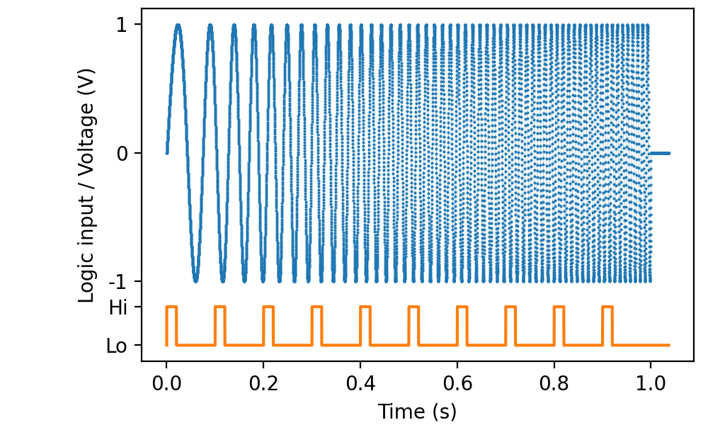
Then we connect do0 to di0 and ao0 to ai0 to verify that the result is as expected:
with AnalogOut(rate=fs) as ao:
    with DigitalOut() as do:
        with AnalogIn(channel=0) as ai:
            with DigitalIn(line=0) as di:
                ao[0].sampled(vv, scale=1*V)
                do[0].stimulus(train)
                ao.run()
                data, times = ai.readall(times=True)
                ddata = di.readall()

plt.plot(times, data, '.-', markersize=1, linewidth=0.1)
plt.plot(times, -1.5 + .3*ddata)
plt.xlabel('Time (s)')
plt.ylabel('Logic input / Voltage (V)')
plt.yticks([-1.5, -1.2, -1, 0, 1], ['Lo', 'Hi', -1, 0, 1])